


Sector Volatility Unveiled: Calculating Implied Volatility and Its Sector-Specific Impact
A short study to see the contribution of implied volatility in option pricing, interpretation of IV curves , comparison of VIX trends.

Implied volatility (IV) is one of the most talked-about metrics in financial markets, especially when it comes to options trading. But what exactly is implied volatility, and how is it calculated? In this article, we’ll break it down in simple terms and explain how the Black-Scholes-Merton (BSM) model is used to calculate IV.
Implied volatility represents the market's expectation of how much the price of an asset (like a stock or an index) will move over a specified period in the future. It's "implied" because it's derived from the current prices of options on that asset, rather than being directly observable in the market like historical volatility.
It provides insight into overall market sentiment—high implied volatility often indicates fear or uncertainty, while low implied volatility suggests a calm or complacent outlook.
How is Implied Volatility calculated?
Implied volatility isn’t something that can be directly observed. Instead, it's inferred from the prices of options using models like the Black-Scholes-Merton (BSM) formula.
The BSM formula is designed to give the theoretical price of an option based on these inputs. However, implied volatility is the one missing piece of information that can’t be directly plugged into the formula. It’s the only variable that needs to be “solved” for by adjusting it until the theoretical option price matches the actual market price.
The Black-Scholes-Merton (BSM) Model for Implied Volatility
The Black-Scholes-Merton model is a widely used mathematical model for pricing European-style options. The formula is:
Where:
C = Call option price
S = Current stock price
K = Strike price of the option
T = Time to expiration (in years)
r = Risk-free interest rate
N() = Cumulative distribution function of the standard normal distribution
d_1 and d_2 are intermediate calculations:
\(d_1=\frac{ln(S/K)+(r+σ^2/2)T}{σ\sqrt{T}} \)\(d_2=d_1 − σ \sqrt{T} \)
σ = Volatility (what we are trying to calculate)
The BSM formula gives us the theoretical price of an option based on the inputs above. But in the real world, the option price is determined by the market, which may be higher or lower than the theoretical value. To find the implied volatility, one solves the BSM formula backward, adjusting σ (volatility) until the theoretical price equals the market price of the option.
IV CURVES AND THEIR IMPLICATIONS
We discuss two types of IV curves:
1. IV Curve vs. Time to Expiration
2. IV Curve vs. Moneyness
Implied volatility (IV) is a key metric for understanding how options traders are pricing risk. But implied volatility isn’t constant! It varies based on two crucial factors: time to expiration and moneyness (the relationship between an option’s strike price and the underlying asset's current price). We explore how these two factors influence IV and how plotting them as IV curves can provide valuable insights into market sentiment and options pricing strategies.
Both curves reveal important information about market conditions, volatility expectations, and potential price movements.
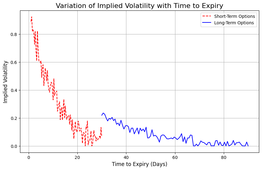
IV Curve vs. Time to Expiration
While plotting implied volatility against
Characteristics:
Short-Term Options: As expiration nears, implied volatility tends to rise, especially in the final days leading up to expiration. This is generally due to the increased uncertainty or the higher probability of significant price movements as time runs out.
Long-Term Options: Longer-dated options generally have lower implied volatility, as the market has more time to absorb potential price movements. However, there may still be periods of elevated IV if the market expects future uncertainty (earnings announcements, geopolitical events etc.).
Example of a Typical IV Curve Over Time:
The volatility curve for longer-term options is often smoother, while shorter-term options may exhibit more pronounced spikes due to immediate risks or upcoming events.
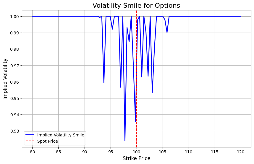
IV Curve vs. Moneyness
The IV curve plotted against moneyness examines how implied volatility varies depending on how far in or out of the money an option is. Moneyness refers to the relationship between the option’s strike price and the current market price of the underlying asset.
Volatility Smile
The particular shape of the volatility smile occurs when implied volatility is higher for both deep ITM and deep OTM options, and lower for ATM options. The resulting graph of implied volatility versus strike price resembles a “smile” shape. Otherwise, under assumptions used in the BSM model, the volatility “smile” would be flat.
Deep In-the-Money Options (ITM): These options have intrinsic value and are more sensitive to the underlying asset's price changes. Because of this, they often show higher implied volatility. Market participants are willing to pay more for hedging in these areas, leading to an increase in IV.
At-the-Money Options (ATM): These options are more dependent on time value and expected volatility. Since the strike price is close to the spot price, there is less uncertainty compared to deep ITM or OTM options, so implied volatility tends to be lower here.
Out-of-the-Money Options (OTM): OTM options, especially deep ones, also tend to have higher implied volatility. Even though these options have no intrinsic value, market participants anticipate that large price movements could bring them into profitability, leading to higher IV.
This pattern of higher IV for both ITM and OTM options is characteristic of the volatility smile.
Volatility Skew
In some markets, especially for equity options, implied volatility doesn’t always follow the smile pattern. Instead, we see a volatility skew, where implied volatility is higher for OTM put options compared to OTM call options.
This may happen because:
Traders are willing to pay more for downside protection (puts) in case of a market crash or significant price drop, especially in bearish or uncertain markets.
In such markets, there is more demand for protection against large price drops, leading to higher implied volatility for puts, while calls might exhibit relatively lower IV.
Code :
https://colab.research.google.com/drive/1t9SVg6_JXbpVeDAnDOZZrh6Hzg_vXEuI?usp=sharing
The above code illustrates the Implied Volatility for the banking industry, where we have taken the top 5 companies (SBI, HDFC bank, ICICI bank, Axis bank, Kotak bank) in the sector based on market cap, for the year 2024 .
The
brentqfunction is an algorithm used to find the root (zero) of a continuous real-valued function. It is part of thescipy.optimizemodule in Python and implements Brent's method, which is a hybrid root-finding algorithm combining the bisection method, secant method, and inverse quadratic interpolation. This combination allows the method to be very reliable and fast.We use the brentq function to backtrack from BSM and find the implied volatility needed.
The
brentqfunction specifically requires that you provide:A function
f(x)where the root (zero) is being sought.Two points
aandbsuch thatf(a)andf(b)have opposite signs, indicating that the root lies between these two points.The graph of the IV shown shows various spikes which may imply
Market Sentiment or Uncertainty
Supply and Demand Imbalance
Upcoming Catalyst or Known Risks
Market Panic or Fear
IV curves interpretation and strategies to implement:
Depending on the market situation the IV curves can show various shapes -
Convex Implied Volatility Curve
Shape: A convex IV curve, on the other hand, would resemble a “U”, with implied volatility higher for ATM options and lower for deep ITM and OTM options.
Interpretation
Market Behaviour: This shape may indicate that the market expects more volatility for options that are closest to the underlying asset's current price. This suggests that market participants anticipate significant movements in the near term, either up or down, with volatility subsiding for extreme strikes.
Possible Reasons: A convex curve could reflect a scenario where traders anticipate short-term price action around the current spot price but expect less movement further away from that price (i.e., lower risk or stability in the tails).
Skew: The convex curve can be a result of demand for ATM options, where investors may be hedging or speculating on near-term volatility but don't foresee substantial tail risks.
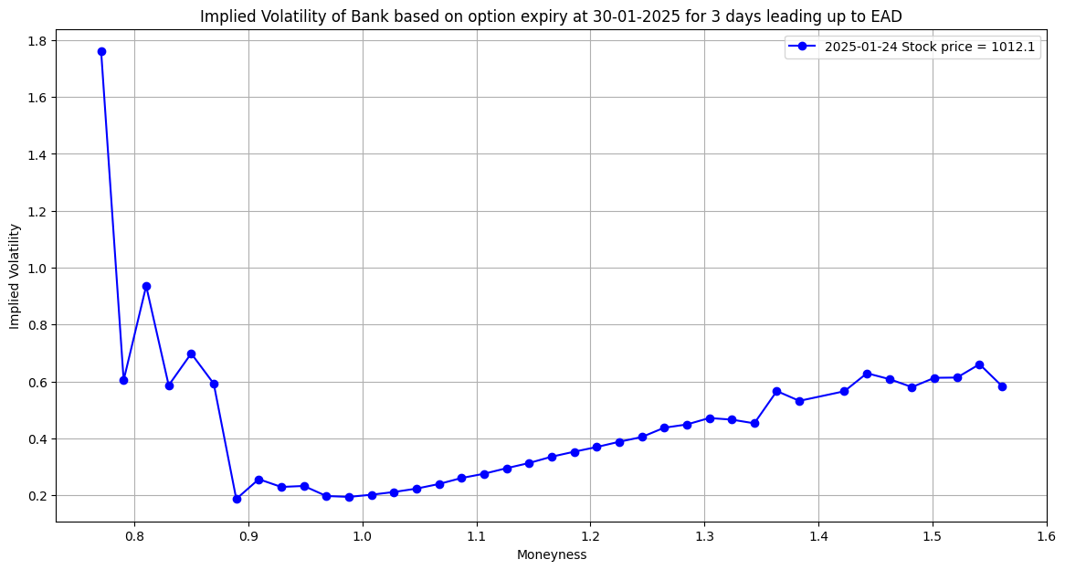
However, earnings announcements are corporate events that provide investors with fundamentally important information. The various facets of the behaviour of stock returns and systematic risk on earnings announcement days (EADs) have been widely studied in academic literature. Investors predict that the news will, more often than not, result in a significant change in either direction of the underlying stock price. Due to the anticipated stock price increase, the ex-ante risk-neutral distribution (RND) displays bi-modality and the implied volatility (IV) curve exhibits concavity. Using data on extremely short-term options, we establish experimentally that bi-modality in the risk-neutral distribution and concavity in the IV curves are ubiquitous characteristics before EADs. The pricing implications of these occurrences are then examined.
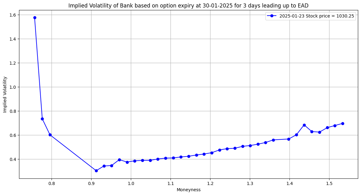
Concave Implied Volatility Curve
Shape: A concave IV curve looks like an inverted “U”, where implied volatility is higher for both deep in-the-money (ITM) and out-of-the-money (OTM) options, and lower for at-the-money (ATM) options.
Interpretation
Market Behaviour: This shape may suggest that traders are expecting more extreme price movements (either up or down), but that the current market outlook for near-the-money options is relatively stable.
Possible Reasons: This can occur in markets with anticipated volatility or uncertainty, such as during periods leading up to significant earnings reports, elections, or economic announcements. It can also occur in markets where participants are seeking protection against tail risks (large market moves).
During this time the premium and volatility for ATM options are the maximum as all investors in market would be using ATM options to hedge their positions to avoid any losses in the extreme market price swing expected to come.
Some strategies that could be used to hedge our position and possibly earn a profit in such a situation is -
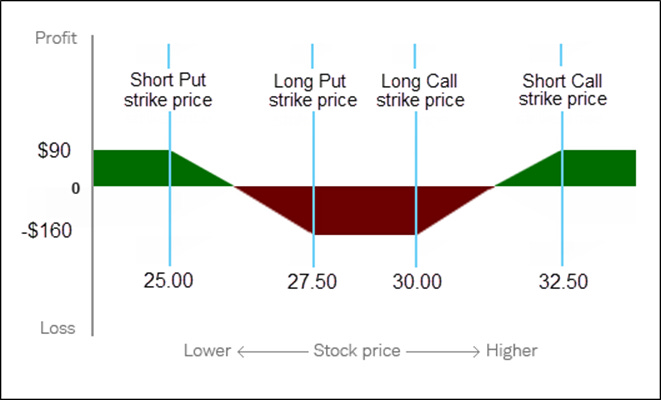
Iron Condor
The short condor involves the following setup:
Sell 1 lower strike call (at the lowest strike price)
Buy 1 middle strike call (higher than the first call)
Buy 1 middle strike put (lower than the highest strike)
Sell 1 higher strike put (at the highest strike price)
This creates a situation where you're short on the wings (the calls and puts at the farthest strikes), while you're long on the two middle options.
Long Straddle
The long straddle involves -
Buy a call option of strike K1
Buy put option of strike K1
Profit: The potential profit is unlimited if the price moves significantly in either direction.
Loss: The maximum loss is limited to the total premium paid for both options (the combined cost of the call and put options)
This strategy benefits from high volatility because the more the asset moves, the higher the chance one of the options will become highly profitable.
IMPMOVE is a measure of the percentage change in the stock price in either direction needed to offset the cost of a symmetric ATM straddle.
Long Strangle
Straddles are structured to benefit from shifts in prices greater than the ATM prices. When prices increase, the resulting change in option value is captured by delta neutral straddles. Price jumps violates this neutrality, if investors anticipate huge jumps in price movements they can suitably use strangles to hedge the gamma risk.
Strangles have a lower cost compared to straddles but, the downside is a price change in either direction has to be sufficiently large for a strangle to pay off. The further the strikes are apart, the less the downside risk and the farther the stock price has to move for a profit to be realized .
Purchasing an out the money (OTM) call and a put, investors bet there will be a large price move in either direction to the current price. We imply that in the presence of concave implied volatilities prices are very volatile and investors are willing to pay substantial premiums to hedge the risk surrounding earnings.

Additional code used to test IV curves around EAD’s:
https://colab.research.google.com/drive/1TkKvM7YVrWGtgt65PAL_ORMYV-TILnu6#scrollTo=sItNKBzvAmo--
Conclusion
In conclusion, understanding the implied volatility curve and its concavity around expected asset distributions (EADs) is crucial for effectively interpreting market sentiment and risk. The shape of the implied volatility curve provides insights into market expectations regarding future volatility, with particular attention to how it behaves near strikes close to the asset’s current price. This can serve as a signal for traders and risk managers to assess potential volatility trends and adjust their strategies accordingly.
Furthermore, the calculation of EADs and their interaction with implied volatility is a powerful tool for pricing and managing risk. By considering the curve's concavity, we can better understand the nature of the risks associated with different strike prices and time horizons, and optimise our positions in response. Ultimately, interpreting these factors together can lead to more informed decision-making in both trading and risk management contexts, improving the ability to navigate uncertain market conditions.
Authors
Rohan Agarwal
Atharva Agarwal