Modelling Markets, Making Money

A short study of market price distributions, basics of option pricing, limitations and alternative approaches like Variance Gamma.

Jan 23, 2025

Imagine tracking the performance of a stock or index over time. The percentage change in its value—whether over a minute, a day, or a year—is what we call a percentage return. It’s a universal metric for measuring the gain or loss investors experience. Investors care about percentage returns because they provide a straightforward way to evaluate performance, compare assets, and make informed decisions.

Our aim is to model these returns and answer questions like: "What is the probability that NIFTY gives a positive return in the next month?" Unlike predicting exact future values, modelling probabilities allows us to understand the likelihood of various outcomes, enabling better risk management and decision-making (or 20 din mein paisa double).

A good way to quantify these returns is percentage returns, which refers to the percentage change in the value of a financial instrument, such as a stock or index, over a specific period. They measure the gain or loss investors experience and are a key indicator of market performance.

\( \% \text{Return} = \frac{\text{Current Price} - \text{Previous Price}}{\text{Previous Price}} \times 100 \)

Another way to quantify returns is the logarithmic returns approach which gives a smoother representation because of its additive nature.

\({Log Return} = \ln\left(\frac{A_t}{A_0}\right) \)

where A₀ stands for previous stock price and A_tstands for current stock price.

Probability Distributions

Imagine you're at a crowded amusement park, waiting in line for a rollercoaster. Most people are of average height, with only a few being much taller or shorter. If you gathered the heights of everyone in the line, you'd notice a pattern: most people cluster around an average height, with fewer at the extremes. This same idea holds for many things: standardized test scores, the time it takes people to finish tasks, and even measurement errors. In each case, we see a pattern emerging—a smooth, symmetric curve.

This curve is familiar: it’s the bell-shaped normal distribution. But why does it appear in so many different scenarios?

The answer lies in a key idea from probability theory: the Central Limit Theorem (CLT). The most common form of CLT states that when we sum a large number of independent random variables, their sum will tend to follow a normal distribution, regardless of the individual distributions of those variables. Mathematically, if

\(X_1, X_2, ..., X_n \)

are independent random variables with any distribution, their average

\(\bar{X} = \frac{1}{n} \sum_{i=1}^{n} X_i \)

will approximate a normal distribution as n grows large.

The normal distribution is defined by the density function

\(f(x) = \frac{1}{\sigma \sqrt{2\pi}} \exp\left(-\frac{(x-\mu)^2}{2\sigma^2}\right) \)

where:

μ is the mean (the center of the distribution),
σ is the standard deviation (which measures the spread)

For the stock market, this is crucial. The price of a stock is influenced by countless small, independent factors—news, company performance, market sentiment, and individual trades. Each of these factors contributes a small change to the stock's price, and when you combine them all, the resulting distribution of returns follows this familiar bell curve.

This isn't just a coincidence. It's a result of how systems with many independent components behave. Whether it's the height of people or the daily returns of a stock, the Central Limit Theorem shows that when many small, independent factors come together, they form a normal distribution.

Enough maths, let us now talk about real numbers. The following is the empirical distribution of NIFTY's daily returns from 2007 to 2024.

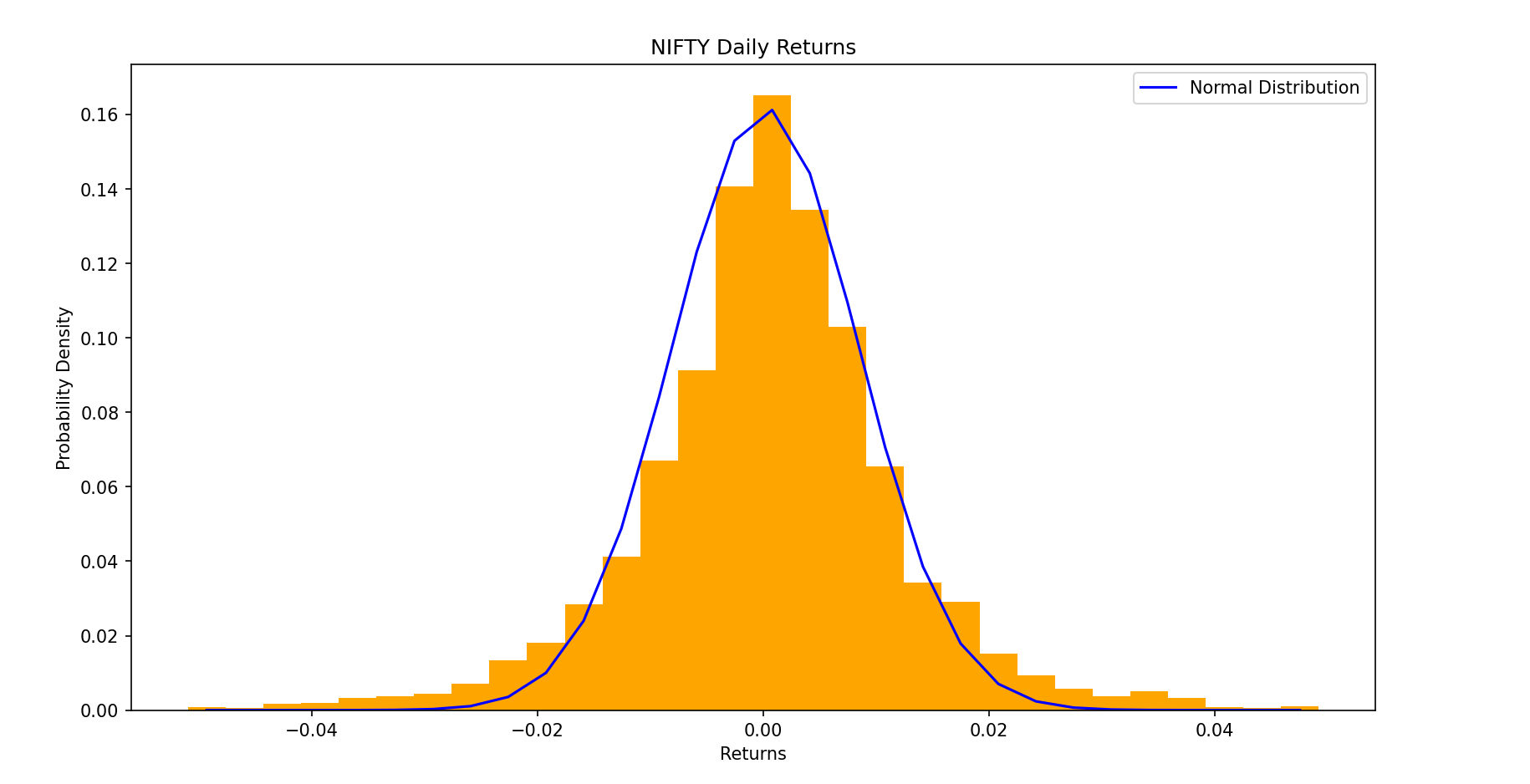
In the image, we see the empirical distribution of NIFTY's daily returns from 2007 to 2024, plotted as a histogram, along with a normal distribution curve for comparison. The histogram shows the actual frequency of returns, while the normal curve represents a theoretical distribution with the same mean and standard deviation. At first glance, the two distributions appear quite similar, especially in terms of their central concentration.

Black-Scholes Model

Imagine a butterfly flying erratically in a field. It moves in random directions, but there's an overall upward drift as it flutters through the air. This is a useful way to think about how stock prices behave over time: erratically, but with a general trend.

To model this kind of behavior, we turn to a stochastic process, where each step is random and independent, but the process evolves in a continuous way. The very meaning of the word stochastic is that can be modelled by some distribution. One of the most famous stochastic processes is the Wiener process, which forms the foundation of models like the Black-Scholes option pricing model.

In the Wiener process, we model the price of an asset as evolving randomly over time. Mathematically, we describe this with the following (stochastic) differential equation:

\(\frac{dS(t)}{S(t)} = \mu dt + \sigma \space dW(t) \)

describes how an asset price evolves over time in the context of Geometric Brownian Motion (GBM), which is a model often used in finance.

μ is the drift rate, also the expected return, which represents how much the asset price is expected to grow on average over a small time interval dt.
σ is the volatility, which measures how much the asset price fluctuates around the expected return.
dW(t) is the increment of a Wiener process (also known as a Brownian motion), which represents the random shocks that drive the price fluctuations. This term is essentially a random noise that varies with time.
S is the current price of the stock while the base price is S₀ .

The point to note here is that we assume dW(t) is normally distributed

\(dW(t)∼N(0,dt)\)

Deriving a distribution for S(t)

Define

\(X(t)=ln⁡(S(t)) \)

Apply Itô's Lemma to find the dynamics of X(t).

\(dX(t) = \frac{1}{S(t)} \, dS(t) - \frac{1}{2S(t)^2} \, (dS(t))^2 \)

Now substitute back the stochastic differential equation

\(dX(t) = \frac{1}{S(t)} (\mu S(t) \, dt + \sigma S(t) \, dW(t)) - \frac{1}{2S(t)^2} (\sigma^2 S(t)^2 \, dt)\)

\(dX(t) = \mu \, dt + \sigma \, dW(t) - \frac{1}{2} \sigma^2 \, dt\)

\( dX(t) = \left( \mu - \frac{1}{2} \sigma^2 \right) dt + \sigma \, dW(t)\)

Integrating both sides

\(X(t) = X(0) + \left( \mu - \frac{1}{2} \sigma^2 \right) t + \sigma W(t) \)

Thus,

\(ln(S(t)) = ln(S(0)) + \left( \mu - \frac{1}{2} \sigma^2 \right) t + \sigma W(t) \)

\(\text{Since } W(t) \sim \mathcal{N}(0, t), \text{ we have:}\)

\(\ln(S(t)) \sim \mathcal{N} \left( \left( \mu - \frac{1}{2} \sigma^2 \right) t, \sigma^2 t \right) \)

Thus, this implies that S(t) is lognormally distributed.

It is easily seen that

\(\ln\left(\frac{S(t)}{S_0}\right) \sim \mathcal{N} \left( \left( \mu - \frac{1}{2} \sigma^2 \right) t, \sigma^2 t \right) \)

The LHS term here is known as the logarithmic return. It is another way of measuring return, just like percentage returns, but possesses favourable properties such as direct additivity of returns (10% down + 10% up is 0).

In contrast to our previous assumption that percentage changes follow a normal distribution, this model implies that the log returns follow a normal distribution.

In finance, the use of log returns makes so much sense, especially while assuming they follow a normal distribution, because stock prices cannot go below zero. Stock prices have a natural lower bound at zero, meaning they cannot become negative.

If we were to assume that percentage changes in stock prices are normally distributed, this could lead to a probability for the stock price becoming negative, which is unrealistic. A normal distribution, with its potential for negative values, would suggest that stock prices could theoretically fall below zero, which isn't possible in practice.

Plotting the empirical distribution using log returns this time gives

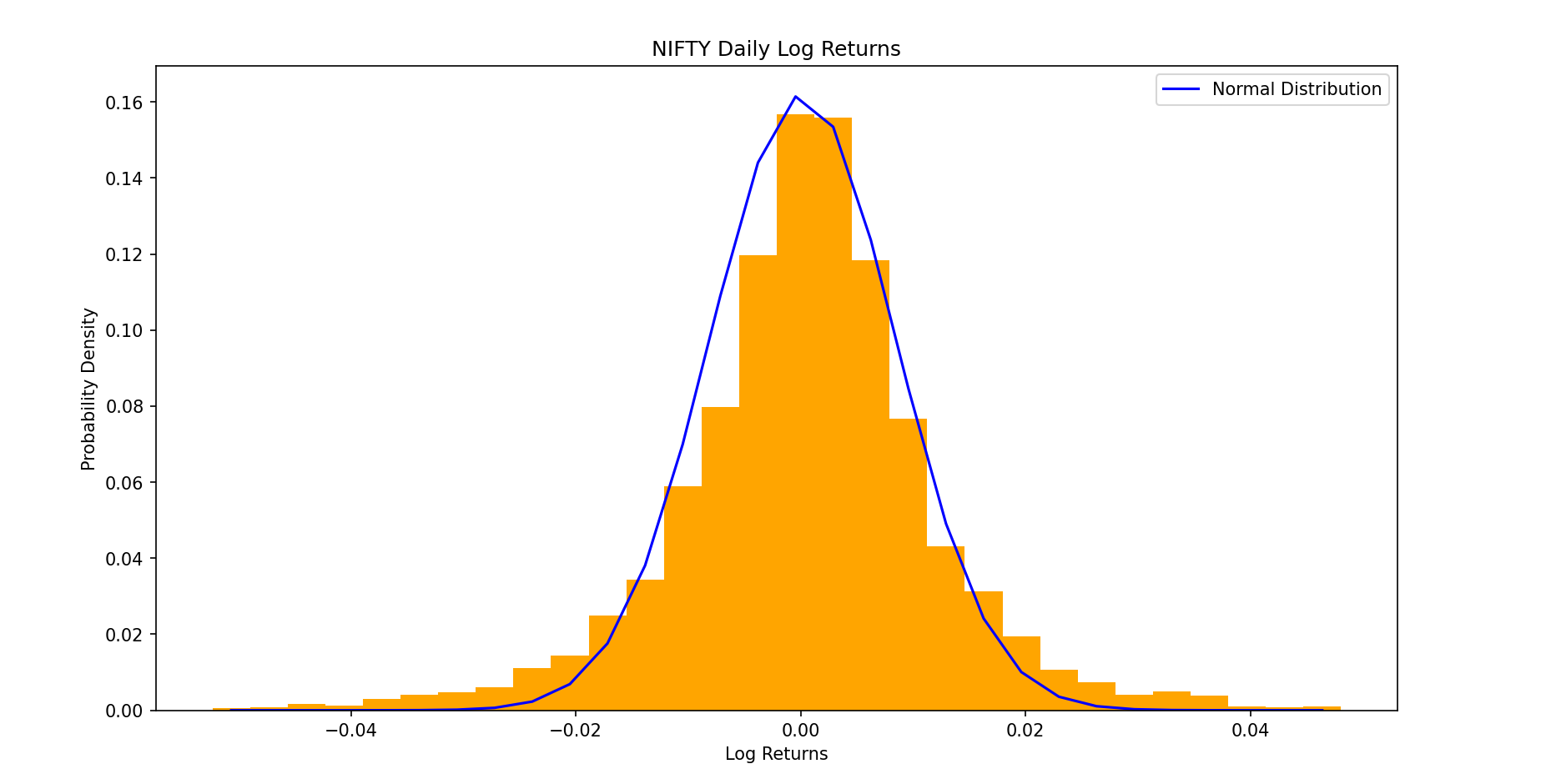
It's evident that the data still exhibits deviations from the ideal lognormal shape. Specifically, the distribution shows signs of skewness, where the data is asymmetrically distributed, and excess kurtosis, indicating the presence of fat tails—a feature not captured by the standard normal or lognormal models.

What Next

There are multiple alternative approaches that try capturing further finer details of returns - the generalised pareto distribution (very good at capturing tail phenomena) and mixture models (aimed at capturing features locally and in ‘globs’) to name a few. Another such approach is to think about time differently.

Stochastic time

Instead of time ticking away evenly like a regular clock, imagine time itself speeds up and slows down randomly. Think of it like this:

On a calm trading day, time moves slowly (few changes).

On a volatile day, time speeds up (lots of changes).

This is where the variance-gamma process comes in. The gamma process governs this randomness. It’s a probabilistic way to stretch or compress time, making the market’s activity more realistic. The Variance Gamma (VG) process provides a way to model stock prices with more flexibility than standard Brownian motion. It accounts for real-world features like asymmetry (skewness) and fat tails (kurtosis).

The Variance Gamma model extends Brownian motion by evaluating a normal process at a random time, which is defined by a gamma process. In simpler terms, the idea is to replace the regular time t in Brownian motion with a time that follows a gamma process, introducing more flexibility in modelling asset prices.

The gamma process has two parameters, μ is the mean rate and ν is the variance rate. The increments of the gamma process over time t to t + h are independent and distributed with a gamma density function:

\(f_h(g) = \left( \frac{\mu}{\nu} \right)^{\frac{\mu^2h}{\nu}} \frac{g^{\frac{\mu^2h}{\nu} - 1}}{\Gamma\left( \frac{\mu^2h}{\nu} \right)} \exp\left( -\frac{\mu}{\nu} g \right) \)

The rigorous derivation of the probability distribution was given by Dilip B Madan, Peter P. Carr and Eric C. Chang in “The Variance Gamma Process and Option Pricing”, 1998.

The expression for the probability density of log returns under the VG process is, rather horrendously, given by

\(h(z) = \frac{2 \exp(\theta x / \sigma^2)}{\nu^{t/\nu}} \frac{1}{\sqrt{2\pi} \sigma \Gamma \left( \frac{t}{\nu} \right)} \frac{x^2}{2\sigma^2/\nu + \theta^2} X^{\frac{t}{2\nu} - \frac{1}{4}} K_{\frac{t}{\nu} - \frac{1}{2}} \frac{1}{\sigma^2} \sqrt{x^2 (2\sigma^2/\nu + \theta^2)}\)

\(x = z - mt - \frac{t}{\nu} \ln(1 - \theta \nu - \sigma^2 \nu / 2)\)

Here, K is the modified Bessel function of the second kind.

The additional parameters, θ and ν give control over the skewness and kurtosis as observed in the empirical plot.

Empirically Fitting the VG Distribution

Fitting the 3 parameters onto the same distribution using the Nelder Method and Log Likelihood , we obtain the following plot

Conclusion

Modelling stock or index returns is essential for evaluating investment performance and making informed decisions. While returns often align with the bell curve of the normal distribution, log returns are preferred in finance due to their non-negativity and additive properties. The Black-Scholes model, based on Geometric Brownian Motion (GBM), assumes lognormally distributed returns, offering mathematical simplicity but failing to capture skewness and fat tails in real data. Advanced models like the Variance Gamma (VG) process address these limitations by introducing stochastic time, where market activity determines the flow of time. This allows the VG model to account for skewness and heavy tails by evaluating Brownian motion at a random time governed by a gamma process. With techniques like Nelder-Mead optimization and log-likelihood fitting, the VG model better aligns with empirical data, effectively capturing real-world market dynamics.

All of this – why? Our larger objective is to be able to accurately predict market price movements (technically called ‘forecasting’), and then use this probability model of ours to price options using exotic and tailored methods – to make money in the derivatives market (subject to terms and conditions).

Authors

Aryan Parekh (Project Lead)

Quant Club’s Substack

Discussion about this post